For each example, I’ll provide Python 3.7 code you can run to see how it all works. You’ll need the TensorFlow library to run the examples. If your GPU supports CUDA, install it with pip ; otherwise use pip . CUDA-accelerated computations are several times faster, so if your GPU supports them, it will save a lot of time. And don’t forget to install the datasets for training with pip .
info
All the examples in this article run completely offline. That’s important because many AI online services—such as those from Amazon—charge per request. By building and training your own neural network with Python and TensorFlow, you can use it without limits and without relying on any provider.
How Neural Networks Work
How does a single neuron work? The input signals (1) are summed (2), with each input having its own weight w. Then an activation function (3) is applied to the result.

This function can be of the following types:
- step (outputs 0 or 1);
- linear;
- sigmoid.
Back in 1943, McCulloch and Pitts showed that a network of neurons can perform various operations. But first, the network has to be trained—tuning each neuron’s w weights so that signals propagate the way we want. Implementing and training a neural network from scratch is hard, but fortunately the necessary libraries already exist. Thanks to Python’s concise syntax, you can do it all in just a few lines of code.
Let’s take a simple neural network and train it to compute the XOR function. Of course, using a neural network to compute XOR isn’t practical. But it’s a convenient way to understand the basics of training and inference and to trace the network’s behavior step by step. Doing this with larger networks would be too complex and unwieldy.
A Simple Neural Network
First, import the required libraries—in our case, tensorflow. I’m also turning off debug logging and GPU usage, since we won’t need them. For working with arrays, we’ll use the numpy library.
import os
os.environ['TF_CPP_MIN_LOG_LEVEL'] = '3'
os.environ["CUDA_VISIBLE_DEVICES"] = "-1"
from tensorflow import keras
from tensorflow.keras import layers
from tensorflow.keras import Sequential
from tensorflow.keras.layers import Conv2D, MaxPooling2D, Flatten, Dense, Dropout, Activation, BatchNormalization, AveragePooling2D
from tensorflow.keras.optimizers import SGD, RMSprop, Adam
import tensorflow_datasets as tfds  # pip install tensorflow-datasets
import tensorflow as tf
import logging
import numpy as np
tf.logging.set_verbosity(tf.logging.ERROR)
tf.get_logger().setLevel(logging.ERROR)
Now we’re ready to build a neural network. Thanks to TensorFlow, it only takes four lines of code.
model = Sequential()
model.add(Dense(2, input_dim=2, activation='relu'))
model.add(Dense(1, activation='sigmoid'))
model.compile(loss='binary_crossentropy', optimizer=SGD(lr=0.1))
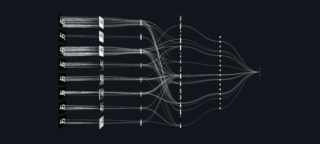
We built a neural network model—the Sequential class—and added two layers: an input layer and an output layer. This type of network is called a multilayer perceptron (MLP); in general form, it looks like this.

In our case, the network has two inputs (the input layer), two neurons in the hidden layer, and a single output.
Let’s see what we’ve got:
print(model.summary())

Training a neural network comes down to finding the values of its parameters.
Our network has nine parameters. To train it, we need a dataset; in our case, it’s the outputs of the XOR function.
X = np.array([[0,0], [0,1], [1,0], [1,1]])
y = np.array([[0], [1], [1], [0]])
model.fit(X, y, batch_size=1, epochs=1000, verbose=0)
The fit function starts the training process, which we’ll run a thousand times; on each iteration, the network’s parameters are updated. Our network is small, so training will be fast. Once training is complete, the model is ready to use:
print("Network test:")
print("XOR(0,0):", model.predict_proba(np.array([[0, 0]])))
print("XOR(0,1):", model.predict_proba(np.array([[0, 1]])))
print("XOR(1,0):", model.predict_proba(np.array([[1, 0]])))
print("XOR(1,1):", model.predict_proba(np.array([[1, 1]])))
The result aligns with what the network was trained on.
Network test:
XOR(0,0): [[0.00741202]]
XOR(0,1): [[0.99845064]]
XOR(1,0): [[0.9984376]]
XOR(1,1): [[0.00741202]]
We can display all the values of the computed coefficients on the screen.
# Parameters layer 1
W1 = model.get_weights()[0]
b1 = model.get_weights()[1]
# Parameters layer 2
W2 = model.get_weights()[2]
b2 = model.get_weights()[3]
print("W1:", W1)
print("b1:", b1)
print("W2:", W2)
print("b2:", b2)
print()
Result:
W1: [[ 2.8668058 -2.904025 ] [-2.871452 2.9036295]]
b1: [-0.00128211 -0.00191825]
W2: [[3.9633768] [3.9168582]]
b2: [-4.897212]
The internal implementation of the model. function looks roughly like this:
x_in = [0, 1]
# Input
X1 = np.array([x_in], "float32")
# First layer calculation
L1 = np.dot(X1, W1) + b1
# Relu activation function: y = max(0, x)
X2 = np.maximum(L1, 0)
# Second layer calculation
L2 = np.dot(X2, W2) + b2
# Sigmoid
output = 1 / (1 + np.exp(-L2))
Consider the case where the network receives the input [0, 1]:
L1 = X1*W1 + b1 = [0*2.8668058 + 1*-2.871452 + -0.0012821, 0*-2.904025 + 1*2.9036295 + -0.00191825] = [-2.8727343 2.9017112]
The ReLU (rectified linear unit) activation function simply replaces negative values with zero.
X2 = np.maximum(L1, 0) = [0. 2.9017112]
The identified values are now passed to the second layer.
L2 = X2*W2 + b2 = 0*3.9633768 +2.9017112*3.9633768 + -4.897212 = 6.468379
Finally, the output uses the Sigmoid function, which squashes values to the 0–1 range:
output = 1 / (1 + np.exp(-L2)) = 0.99845064
We performed the standard matrix multiplication and addition operations and got the result: XOR(.
I recommend experimenting with this Python example on your own. For instance, you can change the number of neurons in the hidden layer. Two neurons, as in our case, are the bare minimum for the network to work.
But the training algorithm used in Keras isn’t perfect: a neural network doesn’t always converge within 1,000 iterations, and the results aren’t always correct. Keras initializes weights randomly, so each run can produce different outcomes. In my case, a two‑neuron network trained successfully only about 20% of the time. When it fails, it looks roughly like this:
XOR(0,0): [[0.66549516]]
XOR(0,1): [[0.66549516]]
XOR(1,0): [[0.66549516]]
XOR(1,1): [[0.00174837]]
That’s not a problem. If you see the neural network isn’t producing correct results during training, you can simply rerun the training algorithm. Once it’s trained properly, you can use the model without limitations.
You can make the network smarter by using four neurons instead of two—just replace the line model. with model.. With this change, the network trains successfully in about 60% of runs, and a network with six neurons trains on the first try about 90% of the time.
A neural network is fully determined by its numerical weights. Once the network is trained, you can save those parameters to disk and then reuse the trained model. We’ll be leveraging this extensively.
Digit Recognition with an MLP
Let’s consider a practical task that’s a classic for neural networks: digit recognition. We’ll use a multilayer perceptron—the same one we used for the XOR function. The inputs will be 28×28 pixel images. This size is chosen because there’s a ready-made dataset of handwritten digits, MNIST, which is stored in exactly this format.
For convenience, we’ll break the code into several functions. The first part is the model creation.
def mnist_make_model(image_w: int, image_h: int):
   # Neural network model
   model = Sequential()
   model.add(Dense(784, activation='relu', input_shape=(image_w*image_h,)))
   model.add(Dense(10, activation='softmax'))
   model.compile(loss='categorical_crossentropy', optimizer=RMSprop(), metrics=['accuracy'])
   return model
The network’s input will take image_w*image_h values — in our case, 28 × 28 = 784. The hidden layer has the same number of neurons: 784.
There’s a quirk with digit recognition. As we saw in the previous example, a neural network’s output can fall in the 0–1 range, while we need to recognize digits 0 through 9. The solution is to build a network with ten outputs, where the output corresponding to the correct digit is set to 1.

The structure of a single neuron is so simple that you don’t even need a computer to use it. Recently, researchers implemented a neural network analogous to our own as a piece of glass—such a network requires no power and contains no electronic components at all.

Once the neural network is created, it needs to be trained. To start, download the MNIST dataset and convert the data into the format the model expects.
We have two data sets: train and test—one is used for training, the other for validating the results. It’s standard practice to train and test a neural network on different data sets.
def mnist_mlp_train(model):
   (x_train, y_train), (x_test, y_test) = keras.datasets.mnist.load_data()
   # x_train: 60000x28x28 array, x_test: 10000x28x28 array
   image_size = x_train.shape[1]
   train_data = x_train.reshape(x_train.shape[0], image_size*image_size)
   test_data = x_test.reshape(x_test.shape[0], image_size*image_size)
   train_data = train_data.astype('float32')
   test_data = test_data.astype('float32')
   train_data /= 255.0
   test_data /= 255.0
   # encode the labels - we have 10 output classes
   # 3 -> [0 0 0 1 0 0 0 0 0 0], 5 -> [0 0 0 0 0 1 0 0 0 0]
   num_classes = 10
   train_labels_cat = keras.utils.to_categorical(y_train, num_classes)
   test_labels_cat = keras.utils.to_categorical(y_test, num_classes)
   print("Training the network...")
   t_start = time.time()
   # Start training the network
   model.fit(train_data, train_labels_cat, epochs=8, batch_size=64,
verbose=1, validation_data=(test_data, test_labels_cat))
Ready-to-use code for training the network:
model = mnist_make_model(image_w=28, image_h=28)
mnist_mlp_train(model)
model.save('mlp_digits_28x28.h5')
We create a model, train it, and save the result to a file.

On my Core i7 machine with a GeForce 1060, the process takes 18 seconds, or 50 seconds without GPU acceleration—almost three times longer. So if you plan to experiment with neural networks, a good graphics card is highly recommended.
Now let’s write a function that recognizes an image from a file—the very thing this network was built for. To perform recognition, we need to convert the image to the same format: a 28×28 grayscale image.
def mlp_digits_predict(model, image_file):
   image_size = 28
   img = keras.preprocessing.image.load_img(image_file, target_size=(image_size, image_size), color_mode='grayscale')
   img_arr = np.expand_dims(img, axis=0)
   img_arr = 1 - img_arr/255.0
   img_arr = img_arr.reshape((1, image_size*image_size))
   result = model.predict_classes([img_arr])
   return result[0]
Using the neural network is now quite straightforward. I created five images with different digits in Paint and ran the code.
model = tf.keras.models.load_model('mlp_digits_28x28.h5')
print(mlp_digits_predict(model, 'digit_0.png'))
print(mlp_digits_predict(model, 'digit_1.png'))
print(mlp_digits_predict(model, 'digit_3.png'))
print(mlp_digits_predict(model, 'digit_8.png'))
print(mlp_digits_predict(model, 'digit_9.png'))

The result, unfortunately, isn’t perfect: 0, 1, 3, 6, and 6. The neural network correctly recognized 0, 1, and 3, but confused 8 and 9 with the digit 6. Of course, you can adjust the number of neurons and the number of training iterations. And these digits weren’t handwritten, so a 100% success rate was never guaranteed.
A neural network like this, with an extra layer and more neurons, correctly recognizes the digit eight, but it still confuses 8 and 9.
def mnist_make_model2(image_w: int, image_h: int):
   # Neural network model
   model = Sequential()
   model.add(Dense(1024, activation='relu', input_shape=(image_w*image_h,)))
   model.add(Dropout(0.2))  # rate 0.2 - set 20% of inputs to zero
   model.add(Dense(1024, activation='relu'))
   model.add(Dropout(0.2))
   model.add(Dense(10, activation='softmax'))
   model.compile(loss='categorical_crossentropy', optimizer=RMSprop(),
            metrics=['accuracy'])
   return model
If you want, you can train a neural network on your own dataset, but you’ll need quite a lot of data (MNIST has 60,000 digit samples). Feel free to experiment on your own; we’ll move on and look at convolutional networks (CNN, Convolutional Neural Network), which are more effective for image recognition.
Digit Recognition with a Convolutional Neural Network (CNN)
In the previous example, we treated a 28×28 image as a simple one-dimensional array of 784 values. That approach works in general, but it starts to fail if the image is shifted, for example. Just move the digit toward a corner in the previous example, and the program will no longer recognize it.
Convolutional networks are much more efficient in this respect: they use the convolution operation, where a so‑called kernel slides across the image and extracts key features when they’re present. The resulting activations are then passed to a “regular” neural network, which produces the final output.
def mnist_cnn_model():
   image_size = 28
   num_channels = 1  # 1 for grayscale images
   num_classes = 10  # Number of outputs
   model = Sequential()
   model.add(Conv2D(filters=32, kernel_size=(3,3), activation='relu',
            padding='same',
input_shape=(image_size, image_size, num_channels)))
   model.add(MaxPooling2D(pool_size=(2, 2)))
   model.add(Conv2D(filters=64, kernel_size=(3, 3), activation='relu',
            padding='same'))
   model.add(MaxPooling2D(pool_size=(2, 2)))
   model.add(Conv2D(filters=64, kernel_size=(3, 3), activation='relu',
            padding='same'))
   model.add(MaxPooling2D(pool_size=(2, 2)))
   model.add(Flatten())
   # Densely connected layers
   model.add(Dense(128, activation='relu'))
   # Output layer
   model.add(Dense(num_classes, activation='softmax'))
   model.compile(optimizer=Adam(), loss='categorical_crossentropy',
            metrics=['accuracy'])
   return model
The Conv2D layer performs a convolution of the input image with a 3×3 kernel, and the MaxPooling2D layer performs downsampling—reducing the image size. At the network’s output, we see the familiar Dense layer that we used earlier.
As in the previous case, the network needs to be trained first; the principle is the same, except that here we’re working with two-dimensional images.
def mnist_cnn_train(model):
   (train_digits, train_labels), (test_digits, test_labels) = keras.datasets.mnist.load_data()
   # Get image size
   image_size = 28
   num_channels = 1  # 1 for grayscale images
   # re-shape and re-scale the images data
   train_data = np.reshape(train_digits, (train_digits.shape[0], image_size, image_size, num_channels))
   train_data = train_data.astype('float32') / 255.0
   # encode the labels - we have 10 output classes
   # 3 -> [0 0 0 1 0 0 0 0 0 0], 5 -> [0 0 0 0 0 1 0 0 0 0]
   num_classes = 10
   train_labels_cat = keras.utils.to_categorical(train_labels, num_classes)
   # re-shape and re-scale the images validation data
   val_data = np.reshape(test_digits, (test_digits.shape[0], image_size, image_size, num_channels))
   val_data = val_data.astype('float32') / 255.0
   # encode the labels - we have 10 output classes
   val_labels_cat = keras.utils.to_categorical(test_labels, num_classes)
   print("Training the network...")
   t_start = time.time()
   # Start training the network
   model.fit(train_data, train_labels_cat, epochs=8, batch_size=64,
        validation_data=(val_data, val_labels_cat))
   print("Done, dT:", time.time() - t_start)
   return model
All set. We create the model, train it, and save it to a file:
model = mnist_cnn_model()
mnist_cnn_train(model)
model.save('cnn_digits_28x28.h5')
Training a neural network on the same MNIST dataset of 60,000 images takes 46 seconds with NVIDIA CUDA and about five minutes without it.
Now we can use a neural network for image recognition:
def cnn_digits_predict(model, image_file):
   image_size = 28
   img = keras.preprocessing.image.load_img(image_file,
target_size=(image_size, image_size), color_mode='grayscale')
   img_arr = np.expand_dims(img, axis=0)
   img_arr = 1 - img_arr/255.0
   img_arr = img_arr.reshape((1, 28, 28, 1))
   result = model.predict_classes([img_arr])
   return result[0]
model = tf.keras.models.load_model('cnn_digits_28x28.h5')
print(cnn_digits_predict(model, 'digit_0.png'))
print(cnn_digits_predict(model, 'digit_1.png'))
print(cnn_digits_predict(model, 'digit_3.png'))
print(cnn_digits_predict(model, 'digit_8.png'))
print(cnn_digits_predict(model, 'digit_9.png'))
The result is much more precise—as expected: [.
All set! You now have a program that can recognize digits. Thanks to Python, the code will run anywhere—on both Windows and Linux. If you want, you can even run it on a Raspberry Pi.
You’re probably wondering if you can recognize letters the same way. Yes—you just need to increase the number of outputs in the network and find a suitable set of training images.
I hope you’ve got enough information to run your own experiments. It’s much easier to figure things out when you have a real example in front of you.