Monitor and Control: How to Audit and Track Everything on Your Linux System

Be Your Own Big Brother

What do we actually mean by “monitoring”? Since my background is in chemical engineering, the term makes me think of industrial process control systems. In essence, you track a set of parameters in a complex system and, based on what you see, you can apply a control action if needed—for example, lower the pressure in a reactor. You can also send a notification to an operator, who will then independently make the appropriate control decision.

For people who aren’t into chemistry but are deep in IT, the picture is a bit different yet familiar: a screen crammed with graphs where some kind of magic happens, like in a Hollywood show. For many admins, that’s exactly how it looks—Graphite/Icinga/Zabbix/Prometheus/Netdata (take your pick) render a slick dashboard you can stare at thoughtfully while idly stroking your beard and smoothing down your sweater.

Most of these systems work the same way: you install so-called agents (collectors) on the endpoint nodes you want to monitor, and then everything runs in either a push or pull model. Either you point the agent to a master node, and it periodically sends reports and heartbeats there; or, conversely, you add the node to the monitoring list on the master, and the master itself goes out and polls the agents for their current status.

No, I’m not going to dive into step-by-step setup guides for these systems. Instead, we’ll roll up our sleeves and get to the bottom of what’s actually happening on the system. By the way, there’s a solid list of tools for sysadmins in Evgeny Zobnin’s article “Sysadmin must-have.” I highly recommend taking a look.

Averages Can Be Misleading

One of the most basic metrics is often covered in the very first Linux lessons—even in schools. It’s the well-known uptime, i.e., how long the system has been running since the last reboot. The utility that reports it is called the same and prints an entire line of useful information:

First you see the current time, then the system’s uptime, then the number of users logged in, and finally the load average—the three mysterious numbers people love to ask about in interviews. By the way, there’s also the w command, which shows the same line plus a bit more detail about what each user is doing.

You can also check uptime directly in /proc, though it’ll be a bit less human-readable in that form:

Here, the first number is how many seconds the system has been running since boot, and the second is how many of those seconds it spent idle, essentially doing nothing.

Let’s take a closer look at the load average—there’s a gotcha here. Let’s look at the numbers again, this time via the /proc interface (the numbers are the same; only the way we obtain them differs):

You can easily find that, in UNIX systems, these numbers are the load averages: the average number of processes waiting for CPU resources, calculated over three time windows leading up to now—1, 5, and 15 minutes. Next, the fourth column shows, separated by a slash, the number of processes currently running and the total number of processes in the system, and the fifth is the last PID the system handed out. So what’s the catch?

Here’s the catch: that holds for UNIX, but not for Linux. At first glance everything seems fine: if the numbers go down, load is decreasing; if they go up, it’s increasing. If it’s zero, the system is idle; if it equals the number of cores, that suggests ~100% load; if you see tens or hundreds… wait, what? Strictly speaking, Linux counts not only processes in the RUNNING state but also those in UNINTERRUPTIBLE_SLEEP—i.e., blocked in kernel calls. That means I/O can drive those numbers, and not just I/O, because kernel calls aren’t limited to I/O. I’ll stop here; for more details, see these two articles: “Как счи­тает­ся Load Average”, “Load Average в Linux: раз­гадка тай­ны”.

Back to our measurements. To see which PIDs are assigned to processes, you can use pidstat and htop (from the htop package—an advanced take on top that shows a ton of information, roughly analogous to a graphical task manager).

In addition, the time command lets you run a process while measuring how long it takes—more precisely, it reports three different times:

As I mentioned above, any program can spend different amounts of time in kernel space and user space—that is, making kernel calls or running its own code. So even a quick look at these numbers can sometimes highlight a bottleneck: if the first metric is much higher, it’s likely an I/O issue; if the second is higher, you probably have inefficient code paths that deserve deeper profiling.

The third metric, total time—also called wall-clock time or real time—is the actual elapsed time from when the program starts to when it returns control. Note that user time can be much larger than real time, because it’s calculated as the sum across all CPU cores. If that happens, it usually means the program parallelizes well.

Lastly, to check the utilization of each CPU core individually, use the following command:

If you see a big skew in per-core CPU load, it means one of the programs actually parallelizes very poorly. And a value of 1 means “refresh once per second.”

Better Than a Goldfish’s Memory

In both science and engineering, the same “problem” keeps popping up: you can’t just give a straight answer to what seems like a simple question. There are nuances and subtleties, and the person asking gets annoyed: “Spare me the details—just give me a number.” Then they get stuck when it turns out different tools report completely different figures—for something as basic as a file’s size or the amount of available RAM…

Speaking of RAM. Since this is hardware we’re dealing with, the first thing we can do is brazenly head over to /proc again:

…and you’ll get a ton of numbers, most of which aren’t particularly meaningful, since that’s basically every RAM metric the kernel exposes. So it’s better to stick with the good old free command:

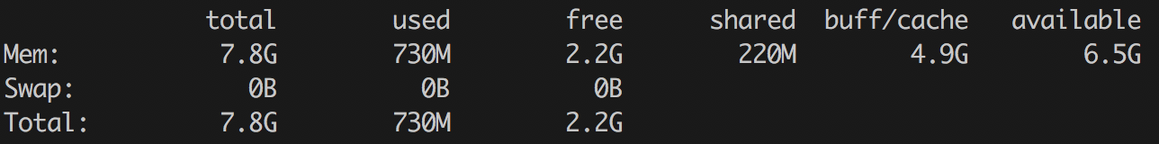
By the way, why aren’t we getting RAM info from /sys, like I described in the sidebar? Because “screw you, that’s why.” Here’s a short note that explains where memory lives in /sys and how to work with it: How memory is represented in sysfs. In short—you’ll need to do some mental multiplication and read a bunch of different files.

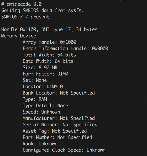
Surprisingly, you can get even lower-level RAM details than /proc/meminfo provides using the dmidecode utility (from the package of the same name). It talks directly to the BIOS and can even report vendor/manufacturer names—though they aren’t always accurate (it’s especially entertaining to run it under a hypervisor, but that’s another story).

By the way, top and htop—like the plain old ps aux—also report memory usage, and htop even draws an ASCII graph for memory and CPU cores. In color. Lovely.

The first two columns are self-explanatory:

• PID — process ID;
• User — the user the process runs as.

And the next two are a bit more interesting: Priority and Niceness, with the former generally equal to the latter plus 20. Essentially, Priority shows the process’s absolute priority in the kernel, while Niceness is relative to zero (zero is usually the default). This priority is factored in when the scheduler hands out CPU time slices, so, strictly speaking, by raising a process’s priority with the renice command you can make a very CPU‑bound task run a little faster. For real-time processes, the Priority column will show rt, i.e., real time—“ASAP.”

The following are the memory details:

• VIRT — virtual memory “promised” to the process by the OS (its total virtual address space, including mappings that aren’t necessarily resident).
• RES — resident memory actually in RAM. Note: due to copy-on-write, you can have N forks of the same process each showing the same value M in this column; that doesn’t mean N×M RAM is consumed, because those pages are shared until they’re modified.
• SHR — shared memory, i.e., memory that can be shared between processes (e.g., for inter-process communication and shared libraries).

And the most basic metrics:

• CPU% — the percentage of CPU the process is using; can exceed 100% if it runs across multiple cores.
• MEM% — the percentage of memory consumed by the process.
• TIME+ — total CPU time the process has used so far.
• COMMAND — the command line (program plus arguments) that was executed.

But we want to go even deeper—we need more details!

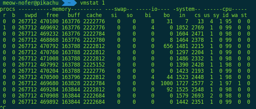
There are lots of columns here as well; to keep it simple, we’ll look at four:

• r — run queue length (number of runnable processes waiting for CPU)
• b — number of processes in uninterruptible sleep
• si/so — number of pages being swapped in from disk / swapped out to disk right now

Do we need to explicitly state that, in a perfect world, they should be set to zero?

Where to Keep Your Lute Music Collection

If you’ve ever manually partitioned a disk (for example, while installing Arch Linux), you probably know the fdisk utility. It’s the easiest way to view the partitions on that disk:

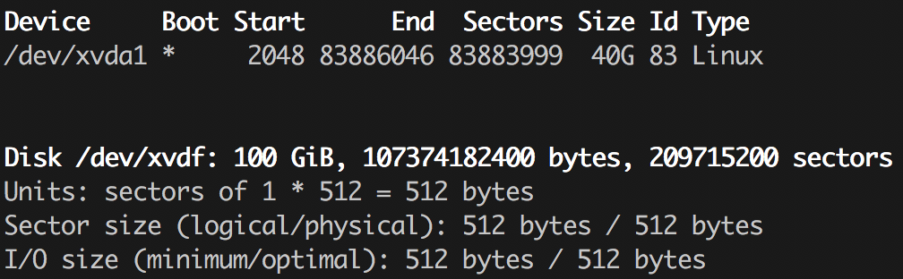
There’s a more full-featured variant with a pseudo-graphical (text UI) interface called cfdisk, plus a couple of other tools that at first glance do similar things—let you manage disk partitions. Those are parted (which, by the way, has a solid GTK GUI in the form of gparted) and gdisk. This ecosystem exists because there are several partitioning schemes, and historically different tools were used for each. You’ve probably seen abbreviations like MBR and GPT. I won’t go deep into the differences; you can read, for example, the article “Срав­нение струк­тур раз­делов GPT и MBR.” It’s discussed from a Windows setup perspective, but the gist is the same. And yes, these days fdisk already уме­ет work with both schemes, as does parted, so the choice mostly comes down to personal preference.

Let’s get back to information gathering. We know which partitions we have, so now let’s look at the filesystem tree—specifically, what’s mounted where:

As before, -h here enables human-readable size output. And, as you remember, you can check file sizes with the du command:

I’m sure some readers are thinking, “What a cliché—even schoolkids know this. Give us something fresher.” Fine, let’s bring in some real-time, like we did with RAM earlier:

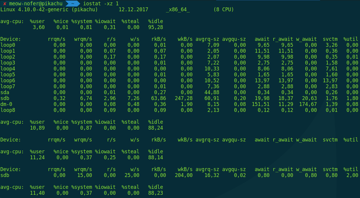
This command displays the average read/write operation counts for all block devices in the system, updating once per second. These are more “hardware-level” metrics, so there’s another command for per‑process I/O statistics, aptly named iotop.

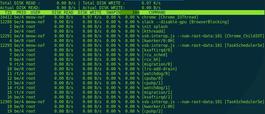
If you try to run it without root privileges, it will politely explain that, due to CVE‑2011‑2494—a bug that can leak potentially sensitive data between users—you should configure sudo. And it’s right.

Want packets with that?

What I/O operations are left? Right—networking. And that’s where things get messy: the “official” tools change from release to release. On the plus side, they keep getting more convenient; on the minus side, you have to relearn them every time.

Say, which utility would you use to view the network interfaces present on a system? Who said ifconfig? On modern systems, ifconfig is typically not even installed anymore, because there’s…

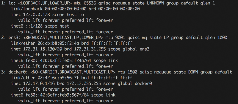
It may look a bit different, but it’s basically the same. By the way, to manage network bridges from the console you often need to install the bridge-utils package. That gives you the brctl utility, which lets you list them (brctl show) and modify them. But sometimes it’s different: I’ve run into cases where the bridges existed, yet brctl didn’t show them. It turned out they were created with Open vSwitch and a custom kernel module, which you configure with a different tool — ovs-vsctl. If you’re in an OpenStack environment, where this is widely used, that tip may be useful.

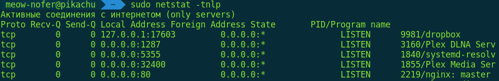
Next—how about routing tables? You say route -n? Nope, not quite. These days it’s more common to use netstat -nr and ip route show. And the obvious one—how do you check open ports and the processes that own them? For example, like this:

But I think you’ve already realized we won’t stop at the basics. Let’s now watch, in real time, how packets move across the interfaces.

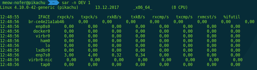
Yes, sar is another excellent monitoring utility. It can show not just network activity, but also disk and CPU activity. You can read more about it, for example, in the article “Simple system monitoring with SAR.”

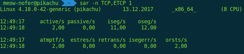
sar also lets you monitor connection opens/closes and retransmissions in real time (i.e., re-sending the same data when network equipment glitches or the link is very unstable—very helpful for troubleshooting).

And lastly—by order, not by importance—is inspecting the network traffic itself. The two most common tools for this are tcpdump and Wireshark. The former is a command-line utility; you can, for example, start capturing on all interfaces and write the traffic to a pcap dump file:

The second one is graphical. From it you can start a capture just the same, or simply open a ready-made packet dump you’ve pulled from a remote server—and revel in the beauty of the protocol stack, the OSI layers (or more precisely, TCP/IP).

Information Is the New Gold

When it comes to computer systems, it’s always better to know than not to know—especially in engineering and infosec. Sure, setting up monitoring with alerts doesn’t take long and pays dividends, but being able to log into a remote server, diagnose the issue from the console in a couple of minutes, and propose a fix—that’s hands-on wizardry few can pull off. Good thing you’ve now got a toolkit for tricks like that, right?