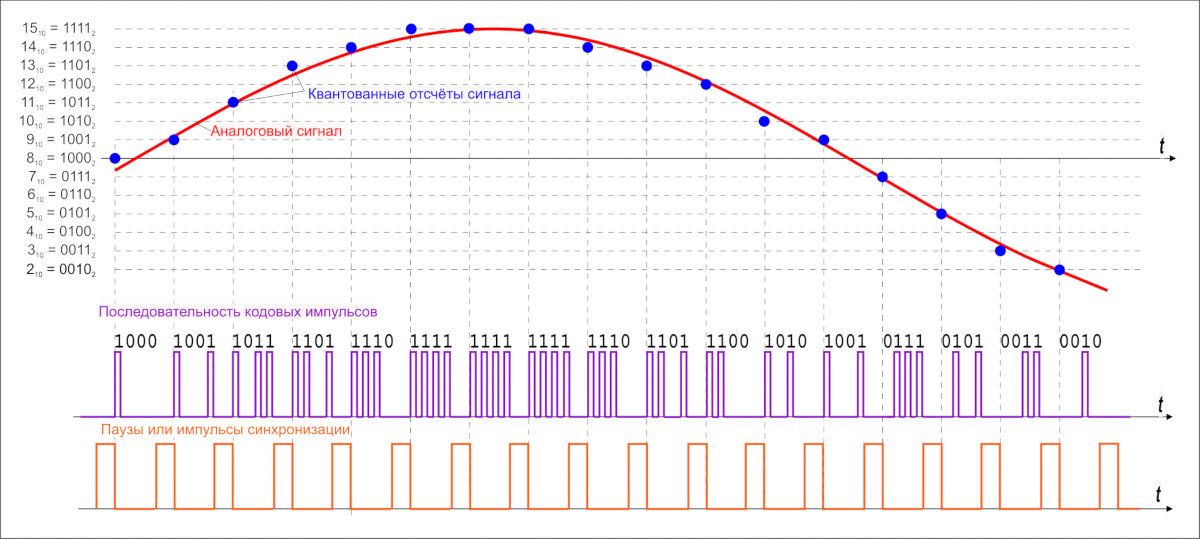
PCM (Pulse‑Code Modulation)
As is well known, in digital audio almost every format, with rare exceptions, is recorded as a pulse-code stream, or PCM stream — pulse code modulation. FLAC, MP3, WAV, Audio CD, DVD-Audio, and other formats are simply ways of packaging—“preserving”—the PCM stream.
How It All Began
The theoretical foundations of digital audio transmission were laid at the dawn of the twentieth century, when researchers tried to send an audio signal over long distances—not by telephone, but by a method that seemed quite unusual for that era.
By slicing the sound wave into small segments, it could be sent to the recipient in a mathematical form. The recipient, in turn, could reconstruct the original wave and play back the recording. The researchers also faced the challenge of increasing the bandwidth of the radio channel.
In 1933, V. A. Kotelnikov’s theorem was published. In Western sources it’s known as the Nyquist–Shannon theorem. Yes, Harry Nyquist was the first to broach the topic: in 1927 he calculated the minimum sampling rate required to transmit a waveform—the quantity later named the Nyquist rate—but Kotelnikov’s theorem was published 16 years before Shannon’s.
The idea is simple: a continuous signal can be represented as an interpolation series of discrete samples, from which the signal can be reconstructed. To approximately recover the original signal, the sampling rate must be at least twice the signal’s upper cutoff frequency.
For many years the theorem wasn’t in demand—until the digital age arrived. That’s when it found practical use. In particular, the theorem proved useful in developing the CDDA (Compact Disc Digital Audio) format, commonly known as Audio CD or the Red Book. The format was introduced by engineers at Philips and Sony in 1980 and became the standard for audio compact discs.
Format specifications:
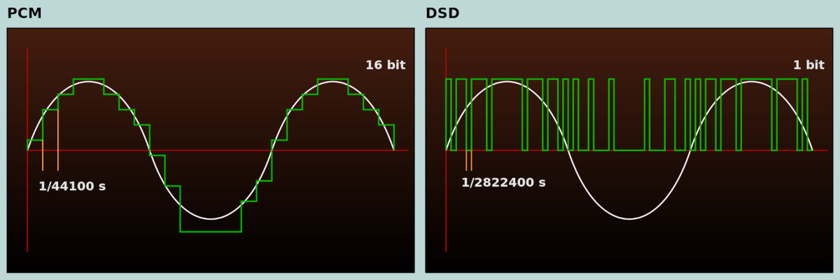
- Sample rate: 44.1 kHz
- Bit depth: 16-bit
info
- – Sampling rate — the number of samples taken per second when digitizing a signal. Measured in hertz.
- – Bit depth — the number of binary digits used to represent the signal’s amplitude. Measured in bits.
The 44.1 kHz sampling rate comes from the Nyquist–Shannon sampling theorem. The average human ear isn’t expected to perceive sounds above roughly 19–22 kHz, so 22 kHz was likely chosen as the upper cutoff, leading to a sampling rate just over twice that.
22,000 × 2 = 44,000 + 100 = 44,100 Hertz
Where did the 100 Hz come from? One theory says it’s a small safety margin for errors or resampling. In fact, Sony chose that rate for compatibility with the PAL TV broadcasting standard.
CDDA uses a 16‑bit bit depth—65,536 quantization levels—which translates to a dynamic range of roughly 96 dB. That many levels were chosen deliberately: first, to keep quantization noise low; second, to ensure a nominal dynamic range higher than the main competitors of the time—cassette tapes and vinyl records. I’ll cover this in more detail in the section on digital‑to‑analog converters.
PCM kept evolving essentially by doubling. New sampling rates appeared: first 48 kHz, and later the derivatives 96, 192, and 384 kHz. The 44.1 kHz family likewise doubled to 88.2, 176.4, and 352.8 kHz. Bit depth grew from 16 to 24 bits, and later to 32 bits.
After CDDA, the DAT (Digital Audio Tape) format arrived in 1987. It used a 48 kHz sampling rate while keeping the same bit depth (16-bit). Although DAT itself flopped, the 48 kHz rate stuck in recording studios, reportedly because it made digital processing more convenient.
The DVD-Audio format debuted in 1999, supporting up to 5.1-channel (six-channel) audio at 96 kHz/24-bit or two-channel stereo at 192 kHz/24-bit on a single disc.
That same year, the SACD (Super Audio CD) format was introduced, but discs for it didn’t go into production until three years later. I’ll cover this format in more detail in the section on DSD.
These are the primary formats regarded as standard for digital audio recordings on storage media. Now let’s look at how data is transmitted in the digital audio signal chain.
Anatomy of the Digital Audio Signal Chain
During music playback, roughly the following happens: the player, using a codec implemented in hardware or software, decodes a file in the chosen format (FLAC, MP3, etc.) or reads data from a CD, DVD-Audio, or SACD disc, producing a standard PCM data stream. This stream is then sent over USB, LAN, S/PDIF, PCI, and so on to an I2S converter. The converter, in turn, transforms the incoming data into I2S data frames (not to be confused with I2C!).
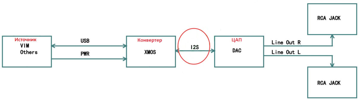
I2S
I2S is a serial digital audio bus. Today it’s the de facto standard for connecting a signal source (such as a computer or media player) to a digital-to-analog converter (DAC). The vast majority of DACs use it, either directly or indirectly. Other digital audio transport standards exist, but they’re much less common.

The I2S bus can have three, four, or even five signals (pins):
- continuous serial clock (SCK) — bit clock (also called BCK or BCLK)
- word select (WS) — frame sync / left‑right clock (also called LRCK or FSYNC)
- serial data (SD) — data line (also labeled DATA, SDOUT, or SDATA). Typically, data flows from the transmitter to the receiver, but some devices can act as both receiver and transmitter simultaneously; in that case, an extra pin may be present
- serial data in (SDIN) — input data line; data flows toward the receiver rather than from it
SD (SDOUT) is the serial data output used to connect a DAC, while SDIN is the serial data input used to connect an ADC to the I2S bus.
In most setups there’s an additional line, the Master Clock (MCLK or MCK). It is used to clock both the receiver and transmitter from a single oscillator to reduce the data error rate. For external synchronization, MCLK is typically derived from two clock oscillators: 22,579 kHz and 24,576 kHz. The first, 22,579 kHz, is for sample rates that are multiples of 44.1 kHz (88.2, 176.4, 352.8 kHz), and the second, 24,576 kHz, is for rates that are multiples of 48 kHz (96, 192, 384 kHz). You may also encounter oscillators at 45,158.4 kHz and 49,152 kHz—by now you’ve likely noticed how the digital-audio world loves powers of two.

I2S requires three lines: SCK, WS, and SD; the other lines are optional.
The SCK line carries the clock pulses that the frames are synchronized to.
The WS line carries the “word” length and also uses logic states. If the WS pin is at logic high, right‑channel data are being transmitted; if it’s low, left‑channel data are being transmitted.
The SD line carries the sample data—the quantized amplitude values (16, 24, or 32 bits). The I2S bus provides no checksums or auxiliary/control channels. If data is lost in transit, there’s no way to recover it.
High-end DACs often include external connectors for I2S. Using those connectors and cables can hurt sound quality—up to audible artifacts and stuttering—depending on the cable’s quality and length. After all, I2S is an on-board interface, and the distance from transmitter to receiver should ideally be near zero.
Let’s look at how a PCM data stream is carried over the I2S bus. For example, with 44.1 kHz PCM at 16-bit resolution, the word length on the SD line is 16 bits, and the frame length is 32 bits (right + left channels). However, transmitters more commonly use a 24-bit word length.

When playing back 44.1 kHz/16-bit PCM, the higher-order bits are either simply ignored because they’re zero-padded, or, with some older multibit DACs, they may carry over into the next frame. The word length (WS) can also depend on the player used for playback as well as the output device’s driver.
As an alternative to PCM and I2S, audio can be recorded in DSD. This format evolved in parallel with PCM, though the Nyquist–Shannon sampling theorem still had some influence here as well. To improve sound quality over CDDA, the emphasis was placed not on increasing bit depth, as in DVD-Audio, but on raising the sampling rate.
DSD
DSD stands for Direct Stream Digital. It has its roots in the labs of Sony and Philips—much like the other formats discussed in this article.
SACD
DSD first appeared on Super Audio CD discs back in 2002.
At the time, SACD seemed like a feat of engineering: it used an entirely new method of recording and playback, one that came very close to analog gear. The implementation was both simple and elegant.
They even added copy protection to the format, though piracy wasn’t really a concern to begin with. Under the Sony and Philips brands, they rolled out “closed” playback-only devices with no way to copy discs. The manufacturers sold recording gear to studios, but kept SACD disc production under their own control.
Who knows—SACD might have become as popular as standard Audio CD if not for the cost of playback hardware. By unjustifiably inflating player prices, Sony and Philips executives undermined their own format’s adoption. Their next misstep effectively killed sales of dedicated players. To help market the PlayStation, Sony’s engineers added SACD playback to the console. Hackers quickly bypassed the console’s protections and started ripping SACDs into ISO images that could be burned to a standard recordable DVD and played on competitors’ players; others simply extracted the tracks for playback on a PC.
Record labels didn’t help either: contrary to audiophiles’ expectations, they failed to leverage what the new high‑resolution format could do. Instead of transferring music to DSD straight from the master tapes, studios often took existing PCM digital masters, remixed them, and ran them through the usual chain—limiters, compressors, dithering with noise shaping, and various digital filters. The result was a sterile, dry sound that could make even Red Book CD seem superior. This undermined listeners’ trust in SACD—and in new formats overall.
info
Sadly, this bad practice is still alive with vinyl: labels press records from digital sources even when they have the master tape. So modern vinyl can easily end up being just 44.1 kHz/16‑bit.
DSD
So what is DSD? It’s a 1‑bit stream with a sampling rate much higher than PCM. DSD uses a different type of modulation, PDM (Pulse Density Modulation). Audio in this format is captured with a 1‑bit analog-to-digital converter; today, sigma‑delta–based ADCs of this kind are used everywhere. The recording process works roughly like this: as long as the waveform’s amplitude is increasing, the ADC outputs a logical 1; when the amplitude is decreasing, it outputs a logical 0. There’s no middle value—it’s always compared against the previous amplitude.
DSD offers several key advantages over PCM:
- More precise waveform reproduction
- Better immunity to interference
- A simpler way to interconnect and transport the digital stream
- In theory, costs could be reduced by simplifying the DAC design, but due to backward compatibility with legacy formats, manufacturers are unlikely to do so
Originally, SACD discs used the DSD x64 format with a sample rate of 2.8224 MHz. It’s derived from the 44.1 kHz Audio CD sample rate multiplied by 64—hence “x64.” Today, the following DSD variants are commonly used:
- x64 = 2,822.4 kHz
- x128 = 5,644.8 kHz
- x256 = 11,289.6 kHz
- x512 = 22,579.2 kHz
- DSD x1024 support is claimed.
DXD
There’s an intermediate format between PCM and DSD called DXD (Digital eXtreme Definition). Essentially, it’s high‑resolution PCM at 352.8 kHz or 384 kHz with 24‑ or 32‑bit depth. It’s used in studios for processing and subsequent mixing.
But that approach is flawed: it doesn’t take advantage of DSD’s strengths, and the files end up larger than DSD. Today’s flagship DACs accept PCM over I2S at sampling rates up to 768 kHz with 32‑bit depth. It’s scary to even think how much hard‑drive space a single album at that resolution would take.
DSD has pretty much split off from SACD. These days you’ll most often see DSD packaged as .dsf or .dff files. There are plenty of players that support DSF and DFF, and audiophiles are increasingly digitizing vinyl in DSD. Recording studios, however, aren’t eager to invest in niche formats, so they keep cranking out audio at the bare minimum: 44.1 kHz/16-bit.
DSD Connectivity and Data Transfer
DSD uses a three-pin connection to carry the digital stream:
- DSD Clock Pin (DCLK) — synchronization (clock)
- DSD Left Channel Data Input Pin (DSDL) — left channel data
- DSD Right Channel Data Input Pin (DSDR) — right channel data
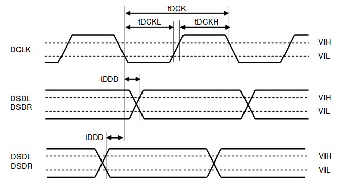
Unlike I2S, DSD data transmission is radically simplified. DCLK defines the bit clock, and the DSDL and DSDR lines carry the left- and right-channel data as serial streams, respectively. There’s no framing trickery here—recording and playback in DSD are strictly bit-by-bit. This approach gets you as close as possible to an analog signal, while the high clock rate reduces quantization noise and improves playback accuracy by roughly an order of magnitude.
DOP
DoP is often used to carry DSD data streams, so it’s worth mentioning. DoP is an open standard for encapsulating DSD data in PCM frames (DSD over PCM). It was designed to allow the stream to be sent through drivers and devices that don’t support native DSD (i.e., non–DSD native).
Here’s how it works: in a 24-bit PCM frame, the top 8 bits are set to all ones, indicating that DSD data is being transmitted. The remaining 16 bits are filled sequentially with the DSD data bits.
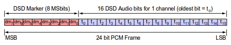
To transmit DSD64 with a 2.8224 MHz 1-bit stream, you need a PCM sample rate of 176.4 kHz (176.4 × 16 = 2.8224 MHz). For DSD128 at 5.6448 MHz, you’ll need a PCM sample rate of 352.8 kHz.
info
For details, see the DoP standard specification (PDF).
Digital-to-Analog Converters (DACs)
Let’s move on to DACs—digital-to-analog converters. It’s a tricky subject, often shrouded in mystery and sprinkled with audiophile mystique. There’s also plenty of hype from opposing camps: marketers, audiophiles, and skeptics. Let’s unpack what’s really going on.
Multibit DACs
In the early days of the Audio CD format, PCM was converted to analog using multibit DACs. These were built around an R–2R resistor ladder with constant impedance.

Multibit DACs work like this: the PCM stream is split into left and right channels and converted from a serial bitstream into a parallel word—typically using shift registers. One register buffer holds the right-channel data, the other holds the left. The data are then output simultaneously over the parallel lines at the chosen sampling rate (most commonly 44.1 kHz), as in the image below—except there are sixteen parallel outputs rather than eight, because the resolution is 16 bits. Depending on their position within the sample word, the most- and least-significant bits encounter different resistance along the current path, since a different number of series resistors are involved. The higher the bit’s significance, the greater its weight in the output.
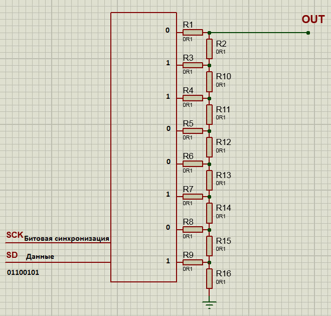
Multibit DACs—often called “multibits”—demand high-quality components and precise resistor matching, because any component tolerances add up. This can cause significant deviations from the original waveform and introduce errors equivalent to several bits of quantization.
Multibit DACs from the 1980s don’t do any PCM trickery. They connect directly to the I2S bus and play PCM as-is: the right channel’s 16 bits arrive, then you wait for the second channel’s 16 bits, and output both channels to the resistor ladder—at a 44.1 kHz rate.
In the 1980s, sampling rate and bit depth were defined by the CD-DA format, which became a near-canonical implementation of the Nyquist–Shannon (Kotelnikov) sampling theorem. With some caveats, the same can be said of the later MP3 format. Only with DVD-Audio did the industry rethink how audio is digitized and reproduced.
That’s how the earliest, simplest DACs worked; later, more sophisticated converter designs were introduced. Circuits were modernized, component quality improved, and multibit DACs started to use oversampling. Oversampling is resampling the digital stream at a higher sampling rate and with greater quantization resolution to reduce quantization noise.
To explain why oversampling is used, we first need to look at how the Nyquist–Shannon (Kotelnikov) sampling theorem works in practice. The real world isn’t as rosy as the math: you don’t get the “arbitrarily accurate” reconstruction the theorem seems to promise.
Nyquist–Shannon Sampling Theorem
“Any function F(t) whose spectrum lies between 0 and f1 can be transmitted continuously, to arbitrary precision, by sending numbers spaced 1/(2 f1) seconds apart.”
Corollaries of Kotelnikov’s theorem:
- Any analog signal can be reconstructed to arbitrary accuracy from its discrete samples taken at a rate f > 2 f_c, where f_c is the highest frequency component within the signal’s spectrum.
- If the signal’s highest frequency is at or above half the sampling rate (the Nyquist frequency), aliasing occurs and it becomes impossible to reconstruct the original analog signal without distortion.
If you’re interested in the details, refer to the original source—the paper “On the Transmission Capacity of ‘Ether’ and Wire in Electrical Communications” by V. A. Kotelnikov (PDF).
The Trouble with the Nyquist Theorem
People often take Kotelnikov’s theorem far too literally and elevate it to an absolute. I’ve read so many articles by hard-headed skeptics praising the “miraculous” MP3 and CDDA formats and mocking audiophiles who try to foist their “unnecessary” DVD-Audio and DSD on everyone. And of course, their go-to argument is Kotelnikov’s theorem (the Nyquist–Shannon sampling theorem).
To start with, simply meeting the Nyquist rate isn’t enough to preserve the exact waveform in practice. Non-ideal conditions inevitably introduce noise and distortion: quantization noise during recording, round-off noise during processing and playback, and more. It’s generally accepted that quantization noise cannot be less than half of one LSB, because the signal is rounded to the nearest quantization level, up or down. Round-off noise likewise can’t be smaller than half an LSB (the quantization step). There are also intrinsic noises in the ADC and DAC, but it’s hard to pin them down precisely since they depend on many factors: the specific design, component quality, and even the environment. Typically, these intrinsic noises amount to a few LSBs.
It follows that the sampling rate should be well above the Nyquist limit to compensate for losses introduced during digitization and subsequent playback.
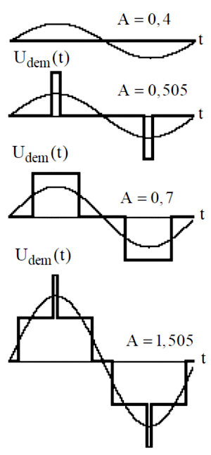
I’ll give an example from E. I. Vologdin’s lecture notes, “Standards and Systems of Digital Audio Recording”:
As you can see, as long as the peak input stays within half a quantization step, the quantizer’s output is zero—a dead zone around zero. This introduces conversion nonlinearity and causes large distortions at low message-signal amplitudes. For A > 1.5, the demodulator output is a train of rectangular pulses whose width varies with the message level. This happens because the quantization errors are on the same order as the input amplitude. The distortion starts to drop noticeably only when A > 2.
Let A denote the signal amplitude.
The quoted passage talks only about quantization noise, assuming the smallest possible value—half a quantization step. Rounding noise has a comparable impact—at least half a quantization step.
Beyond noise, digital recordings can also suffer from artifacts introduced by the LPF—low‑pass filter. According to the Kotelnikov (Nyquist–Shannon) sampling theorem, you must band-limit the audio signal with a filter and treat its cutoff as the highest frequency component; doubling that gives the required sampling rate (the Nyquist rate). The catch is that the theorem assumes an ideal LPF, which doesn’t exist in the real world. Here’s a quote from Vologdin’s lecture notes:
To reliably suppress spectral components above the Nyquist frequency, the anti-aliasing low-pass filter should have a cutoff slightly below Nyquist and provide very strong attenuation (at least 90 dB) at that frequency. In practice, this is typically done with 7th–9th order elliptic filters. The steep roll-off of such LPFs causes characteristic “ringing” distortions. This happens because the impulse response of these filters is an oscillatory sinc-like function. The steeper the roll-off, the slower the ringing decays. The only effective way to mitigate this is to raise the sampling rate, which lets you relax the LPF’s transition steepness without reducing its ability to reject out-of-band components above Nyquist.
Here’s another interesting point. Kotelnikov’s sampling theorem assumes a signal of infinite duration, which conflicts with the practical constraints of recording it to a storage medium or saving it to a file.
Kotelnikov’s theorem gives limiting relationships under idealized conditions—most notably, perfectly band-limited spectra and infinite observation time. Real-world signals are time-limited and have spectra that are not truly band-limited. Modeling a signal as band-limited and observing it over a finite time introduces reconstruction error.
Calculations show that, in practice, the sampling frequency F_D is typically set well above the Kotelnikov (Nyquist) rate. Here, F_D denotes the sampling frequency.
Source — I. P. Yastrebov, “Sampling of Continuous-Time Signals. Kotelnikov’s Theorem” (PDF)
To convey the scale of the problem, here’s another quote.
“Distortions caused by quantization errors are clearly audible even with 8-bit encoding, despite the fact that the distortion level doesn’t exceed 0.5%. This means that with 16-bit encoding, as used for CDs, the actual dynamic range of digital audio doesn’t exceed 48 dB, not 96 dB as the ads claim.”
Source — E. I. Vologdin, “Digital Audio Recording” (PDF)
Conclusions
Kotelnikov’s theorem is mathematically correct, but its practical use needs substantial caveats. The Nyquist rate is better seen as the bare minimum for recovering an approximate waveform, not for reconstructing a signal “with arbitrary accuracy.” To compensate for real-world losses in digitization and playback, the sampling rate should be not just twice, but several times higher than the highest frequency of interest.
With that, let’s set aside the Nyquist–Shannon (Kotelnikov) sampling theorem and move on to the various types of noise that arise during recording, mixing, and playback of an audio signal.
Types of Noise
There are many types of noise that affect a recording. The main ones are: quantization noise, round-off noise, aperture jitter, nonlinear distortion, and analog noise. You can review the descriptions of four types of noise and the formulas to roughly estimate how much distortion each one introduces into a digitized signal.
Don’t think of “noise” here as the familiar “white noise.” Different types of noise are perceived differently; in this context, “noise” is better understood as the loss (or degradation) of part of the useful signal.
You can still roughly estimate a specific type of noise, but gauging the overall noise level during digitization is hardly feasible. The math is complex and full of assumptions. Instead, let’s take the reverse approach: analyze the dynamic range of the signal captured by the ADC (analog-to-digital converter) and compare it to the theoretical maximum.
The noise level is usually referenced to the quantization step (one LSB) or to the dynamic range of the audio signal. The dynamic range is measured in decibels and can be calculated as DR = 20·log10(2N), where N is the bit depth. This gives a theoretical dynamic range of about 96 dB for 16-bit and about 144 dB for 24-bit audio.
Let’s use the results from the test of the Lynx Studio Hilo TB ADC, a high-end studio-grade ADC/DAC. It delivered the following results.
| Operating mode | 24-bit, 44 kHz | |
|---|---|---|
| Dynamic range, dB(A) | 119.3 | Excellent |
Here are the results without enhancement.
| Operating mode | 24-bit, 44 kHz | |
|---|---|---|
| Dynamic range, dB(A) | 112.6 | Excellent |
Jumping ahead, the ADC under test uses dithering, noise shaping, and decimation, which together extend the dynamic range and reduce noise. I’ll cover these techniques in more detail in the next section.
Now, let’s do the math: 24-bit corresponds to 144 dB—that’s the theoretical dynamic range. Subtract the measured 119 dB, and the noise eats up 25 dB in the best case and up to 32 dB in the worst. They didn’t test it at 16-bit, unfortunately, but the ratios would be worse, since reducing bit depth inevitably raises the noise floor. In other words, roughly one-fifth of the signal is simply lost to noise.
The picture isn’t pretty. And if you dig deeper and consider how audio is mixed in a studio, it gets unsettling. A finished track is typically built from samples that already contain the aforementioned noise, because those samples were recorded through similar ADCs. Then effects are added, which at the very least trigger resampling—and with it, rounding errors.
On top of that, bad sound engineers love to crush and flatten everything with limiters and compressors, whose very purpose is to reduce dynamic range. Virtually every sample goes through this torture. Even a simple EQ runs the signal through a digital filter, which adds rounding noise of at least half a quantization step. At final mixdown, all the samples are summed into a single stream, so the noise from each gets added together—plus you pick up the noise from yet another resampling stage. And that’s still not all: during playback, the DAC adds its own noise and rounding error. Imagine what’s actually left of the useful signal.
Noise Reduction Techniques
To address this unfortunate situation, specialized noise-suppression technologies have been developed. Let’s look at the key ones.
Oversampling
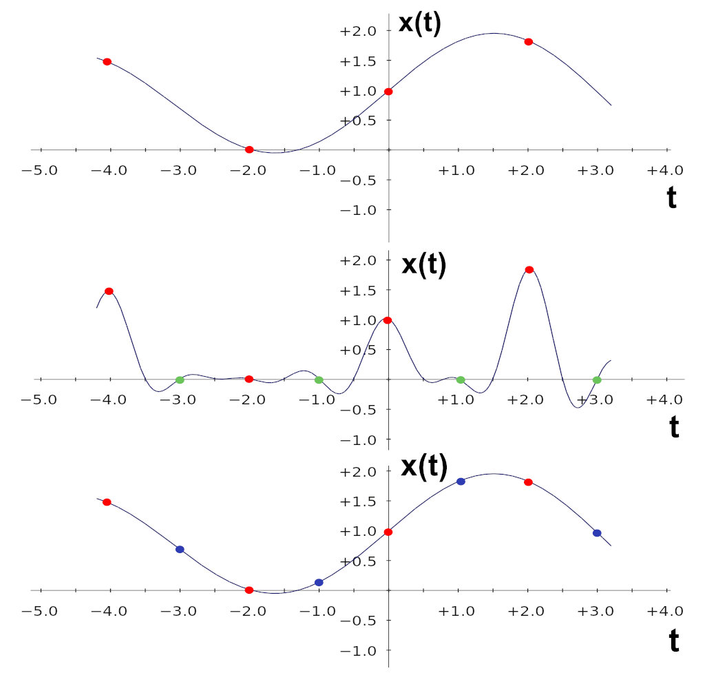
Oversampling has been used since the era of multibit DACs to mitigate noise-related losses. The idea is to insert intermediate samples between the existing ones to approximate the waveform more closely. These intermediate samples are either computed via mathematical interpolation or created by zero-stuffing and then processed by a digital filter. Both approaches are commonly referred to as interpolation, and the digital filter is called an interpolating filter. The simplest form of interpolation is linear interpolation, and the simplest digital filter for this task is a low-pass filter.
Below is an illustration of interpolating a discrete-time signal by a factor of 2. The red dots mark the original samples, and the solid lines show the underlying continuous signal those samples represent. Top: the original signal. Middle: the same signal with zero-inserted samples (green dots). Bottom: the interpolated signal (blue dots are the interpolated sample values).
At first, they used only upsampling—for example, taking 44.1 kHz up to 176.4 kHz. Later, they combined increasing the sample rate with expanding the word length (bit depth)—a process known as requantization.
Although oversampling introduces rounding noise, it expands the signal’s dynamic range, which lowers the overall noise density and makes subsequent processing less impactful. Each doubling of the sampling rate increases the dynamic range by roughly one quantization step—about 6 dB—minus the rounding noise.
To make oversampling feasible, manufacturers began producing multibit DAC chips that accept digital input streams up to 192 kHz/24-bit. Hardware upsamplers based on DSPs (digital signal processors) also emerged.
Of course, using oversampling improved the audio signal’s characteristics, but it didn’t fundamentally change the situation: the noise level was still high. So other techniques started to be used as well.
Decimation (Downsampling)
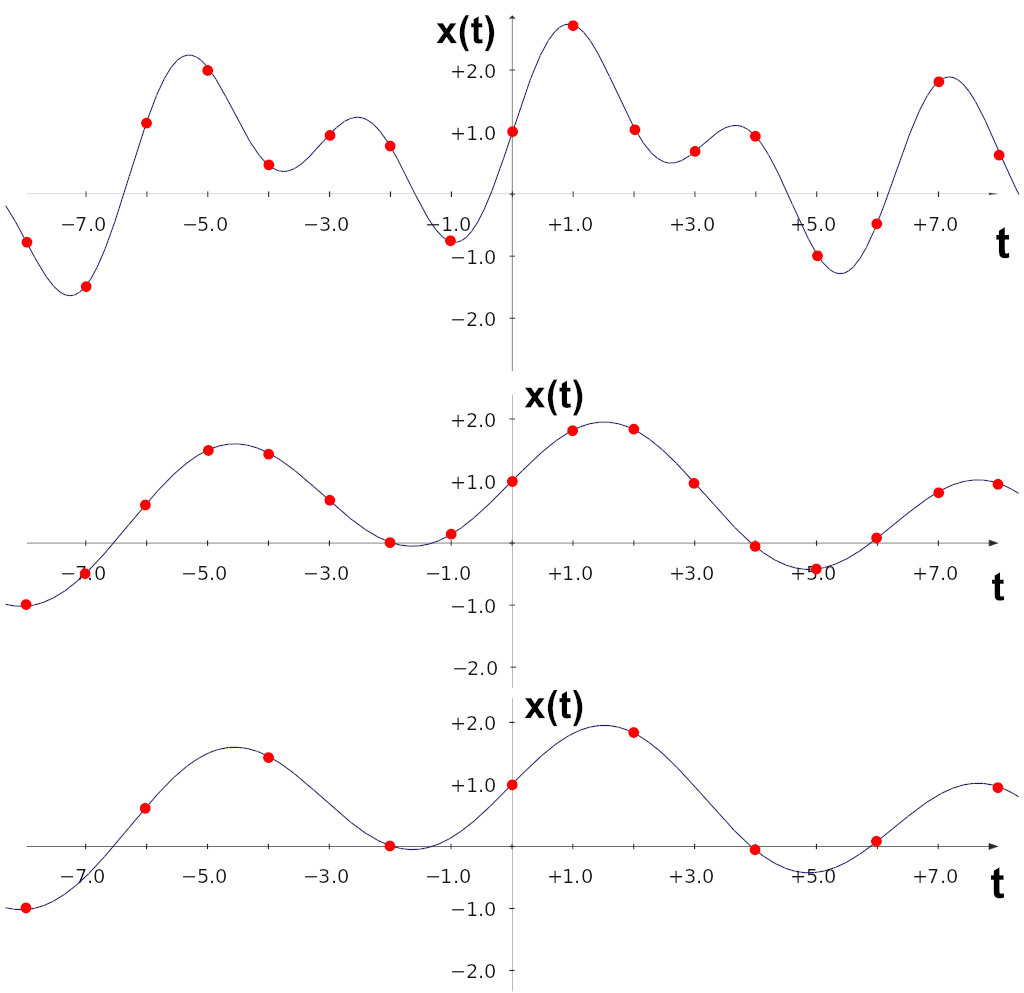
In recording and mixing, engineers began using decimation—essentially resampling downward by reducing both the sampling rate and bit depth. The signal is first captured at a high rate and resolution, for example 176.4 or 192 kHz at 24-bit, and then a digital filter removes some samples to “shrink” it to the CDDA standard of 44.1 kHz, 16-bit. This approach helps slightly reduce quantization noise.
Below is an illustration of decimating a discrete-time signal by a factor of 2. Red dots indicate the samples; solid lines show the underlying continuous-time signal those samples represent. Top: the original signal. Middle: the same signal after filtering with a digital low-pass filter. Bottom: the decimated signal.
Dithering
Dithering — a method of adding pseudo-random noise during the digitization or playback of an audio signal. This technique serves two purposes:
- linearization of the quantizer/requantizer transfer characteristic;
- decorrelation of quantization errors.
Quantization noise is correlated with the program material, which creates spurious harmonics that mirror the signal’s shape. Perceptually, this comes across as a kind of “blur” in the sound. You can remove that correlation by adding a carefully designed dither to the signal, turning the correlated quantization error into ordinary white noise. This slightly raises the overall noise floor but improves perceived quality.

Noise Shaping (NS)
Noise shaping (NS) technology can substantially reduce the noise introduced by quantization, requantization, and dithering.
Noise shaping works like this: the quantized input signal is compared to the requantizer’s output, the difference (the error) is computed, and that error is subtracted from the main signal. This compensates for distortions introduced by the requantizer and by dithering. In effect, you get a feedback loop that tries to cancel the error between the requantizer’s input and output. It’s analogous to negative feedback in an operational amplifier, except all the processing happens in the digital domain.

This technique has its drawbacks. Using noise shaping introduces a lot of high‑frequency noise, so you need a low‑pass filter with a cutoff close to the system’s upper cutoff frequency. In practice, noise shaping is almost always paired with dithering; the combination sounds significantly better.
Dynamic Element Matching
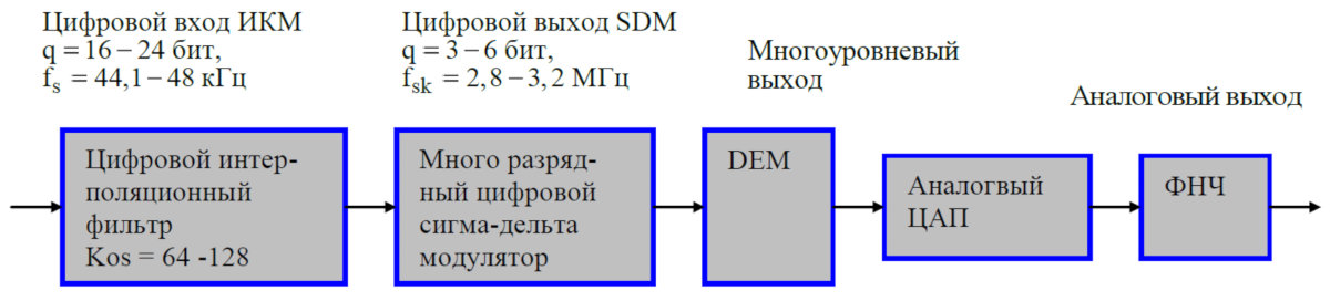
Dynamic Element Matching (DEM) is a technique that makes a DAC produce multiple output levels. It’s essentially a hybrid between a 1‑bit and a multibit DAC. DEM is used to reduce deterministic errors in sigma‑delta modulation (SDM). Like quantization noise, these errors are highly correlated with the output of a 1‑bit modulator, so they can significantly color the perceived audio signal.
This technique also relaxes the requirements for the analog reconstruction filter, because the signal’s shape, even before filtering, is already closer to the final waveform. DEM is implemented using multiple outputs tied together on a common bus, which collectively form the DAC output.
Beyond the techniques already discussed, others are used as well, including various combinations and permutations. Vendors especially like to experiment with digital filtering and modulators, inventing ever-new digital filters that can shape the signal for better or worse. The DSP in modern DACs is typically complex, incorporating all of the above along with each vendor’s proprietary methods. Naturally, manufacturers don’t disclose their filter and modulator algorithms; at best, they share a rough block diagram. As a result, we’re left to infer what actually happens to the audio signal inside any given DAC.
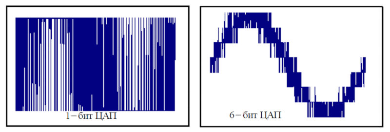
Sigma-Delta DACs
Sigma–delta digital-to-analog converters evolved separately from multibit DACs. As the name implies, they’re based on sigma–delta modulation, commonly abbreviated as SDM. In sigma–delta modulation you don’t transmit the absolute signal amplitude at each instant, as multibit DACs do; instead, you encode how the signal changes relative to the previous value. If the amplitude goes up, you transmit a 1; if it goes down, you transmit a 0. This principle was already described in the section on DSD.
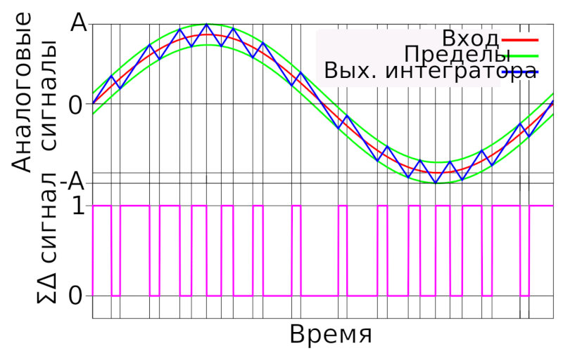
The first delta-sigma DACs were strictly 1-bit, yet thanks to very high oversampling they still delivered a dynamic range of about 129 dB. They used 44.1 kHz as the base sampling rate. That choice likely reduced hardware costs by simplifying the interpolation math.
Initially, a 2.8 MHz rate was used—that’s 44.1 kHz multiplied by 64. Today the rate can vary and is determined by the DAC’s internal architecture. It’s typically based on frequency grids derived from 44.1 kHz or 48 kHz, with multipliers of 64, 128, 256, 512, or 1024.
Over time, delta-sigma DACs have almost completely displaced multibit designs for simple economic reasons. First, they demand much less in terms of component quality and precision than multibit DACs, which lowers manufacturing cost. Second, in the 1980s–1990s the cost of implementing interpolation and noise shaping for a 1-bit modulator was far lower than for 16-bit. Today, with advances in technology, that gap matters less, and many delta-sigma DACs, like multibit ones, use multiple output levels. However, because they operate at much higher sampling rates, the component requirements remain relatively modest, so the first advantage still holds.
Modern sigma–delta DACs have a complex architecture and incorporate nearly all the techniques covered in the previous chapter. Here’s an example of the internal architecture of a simple sigma–delta DAC from Vologdin’s lectures.
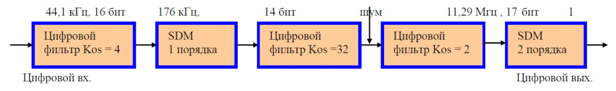
The input consists of 16‑bit digital samples at 44.1 kHz, which are fed to a digital upsampling filter. The design uses a linear‑phase FIR interpolation filter with 4× oversampling. In the first modulation stage, the samples are requantized from 16 to 14 bits and processed by a first‑order sigma‑delta modulator (ΣΔ).
Further oversampling is then performed in two stages with oversampling ratios of 32 and 2. Between these stages, dither at −20 dB is injected to reduce transfer‑function nonlinearity caused by quantization errors. The overall oversampling factor is 256, raising the sampling rate to 11.29 MHz. The second modulation stage employs a second‑order ΣΔ modulator and produces a 1‑bit digital stream. A digital pulse modulator at the DAC output converts this data into a pulse‑density modulated (PDM) sequence.
In short, here’s what happens. The DAC receives a PCM data stream over I2S, performs interpolation (oversampling), adds dither, then feeds it into a feedback requantizer (noise shaping). This produces a 1-bit bitstream that passes through an analog low‑pass filter, where it’s converted into the final audio signal we hear.
A multibit DAC is more complex: in addition to what’s already been covered, it also uses DEM (Dynamic Element Matching) technology.
www
If you want to dive into the details, check the linked resources—they cover not only sigma-delta DACs but also sigma-delta ADCs.
Modern digital-to-analog converters are complex devices. These techniques are used to artificially expand dynamic range, largely to work around the limitations of CDDA and MP3. If recordings were originally released in high-resolution PCM (192/24), or better yet in DSD, there wouldn’t be a need for so many techniques and complex digital conversions. With DSD in particular, you don’t have to manipulate the quantized signal at all—at least during playback.
Conclusion
The path of recording and playback in the digital era has been anything but straightforward. With the advent of the compact disc, analog media virtually disappeared within a couple of decades. Whether that’s good or bad is up to each person, but it would be nice to at least have the option. If not a choice between digital and analog, then at least how and in what quality to listen to your favorite music. Unfortunately, that choice is now almost gone. Today, very few releases come out in high resolution, aside from a handful of enthusiasts on trackers. If there’s anyone to blame, it’s the record labels, which chose to stick with a single format — CD‑DA.
You can’t help but feel for the musicians. They pour so much time and energy into their work, yet the final product often isn’t even preserved in decent quality. Recording to master tape—or at least in DSD—could be a solution. But recording studios won’t go the extra mile; they’re comfortable with the status quo.