
Look at this picture. To answer what it shows, you can describe the scene as a whole. It’s clearly taken outdoors, somewhere in an Asian country. Someone who has been there before might recognize Tiananmen Square in Beijing.
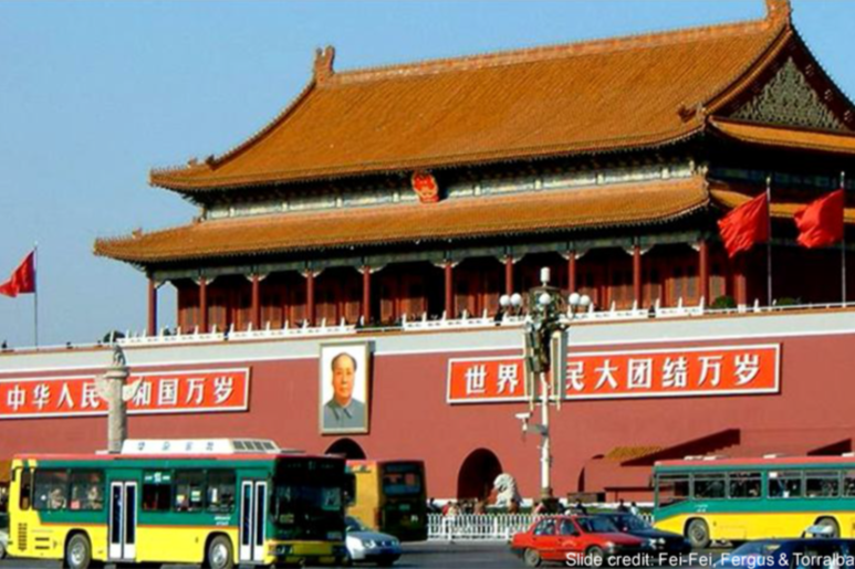
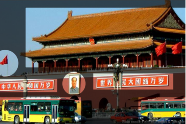
Another approach is to identify individual objects in an image. In the picture you can see a bus, a portrait, a roof, the sky, and so on. You can go further and describe the physical properties of each object. For example, the roof is sloped, the bus is moving and it’s a solid object, there’s an image of Mao Zedong hanging on the wall, and the wind is blowing from right to left (you can infer that from the motion of the flag).
From the example above, we can conclude that answering the question of what’s shown in an image draws on our entire life experience. For example, knowing that wind exists (even though you can’t see it directly in the picture), or what vehicles are. To answer more complex questions, you might even need knowledge of Chinese history. In other words, the task isn’t about looking at pixels—it’s about applying knowledge.
Intra-Class Variability
Let’s take another example. If you ask what a chair is, you might blurt out the first thing that comes to mind: a chair is something with four legs and a backrest. But what about a chair like this?
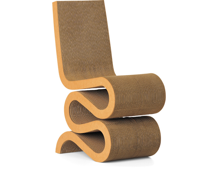
It turns out that even something as simple as a chair is hard to describe purely in terms of shapes. A chair is more of a conceptual category: something you sit on. Imagine trying to explain that to an alien that doesn’t even know what “sitting” is and can’t do it. Before you teach it to recognize chairs in images, it would help if it first understood the concept of sitting.
The same thing happens when you train a computer to recognize images. Ideally, if you want it to answer questions about chairs as well as a human can, it needs to understand the concept of “sitting.”
In AI research, there’s the notion of AI-complete problems—tasks whose solution would essentially amount to creating artificial general intelligence (AGI). General computer vision—being able to say what’s in an image and answer arbitrary questions about it—is considered AI-complete.
We’ve shown that answering a question about an image takes more than just looking—it calls for life experience, education, and sometimes intuition. Unfortunately, artificial general intelligence hasn’t been achieved yet. As a result, computer vision focuses on specific subproblems, which we’ll discuss next.
Computer Vision Tasks
Let’s walk through a few problems that computer vision solves, using examples.
First example: image search on the internet. There are now several services that let you search for pictures. Initially, you searched using text queries. Some time ago, some of these services added reverse image search: you upload an image, and the service looks for similar images on the web.
Here’s how this kind of search works. First, images from the internet are indexed. For each one, a digital representation is computed and stored in a data structure optimized for fast lookup. The same is done for the user’s image: a representation is extracted and used to query the database for duplicates or similar images.
This is a structurally hard problem. The internet hosts billions of images, and using complex comparison methods isn’t feasible because high performance is required.
Here are a few more examples.
Text recognition (OCR). The task is to locate text within an image and convert it into editable, machine-readable content. This technology is widely used across various applications. For example, it’s a convenient way to input text into an online translator: just snap a photo of a label, the text will be recognized, and the translator will produce a translation.
Biometrics. To identify people, systems can use facial images, iris patterns, or fingerprints. That said, computer vision is mostly focused on face recognition. Each year the technology gets better and sees broader adoption.
Video analytics. More and more cameras are being deployed worldwide: on roads to record vehicle traffic, and in public spaces to track people flows and detect anomalies (e.g., unattended items, illegal activity). As a result, there’s a need to process massive volumes of data. Computer vision helps solve this: it can read license plates, identify a vehicle’s make and model, and detect traffic violations.
Satellite imagery analysis. There’s now a massive corpus of satellite images. Leveraging these data, we can tackle a wide range of tasks: improving maps, detecting wildfires, and identifying other issues visible from space. Computer vision has advanced dramatically in recent years, automating more and more of the manual work in this domain.
Graphics editors. Computer vision isn’t just about recognizing what’s in an image; it also lets you modify and enhance it. In that sense, everything you can do with a graphics editor falls under computer vision technology.
3D analysis. 3D reconstruction is another task addressed by computer vision. For example, by using a large collection of photos taken in a city, you can reconstruct the shapes of buildings.
Vehicle control. In the future, every car will be equipped with a vast array of sensors: video cameras, radar, and stereo cameras. Computer vision methods help analyze the data from these sensors and underpin collision-avoidance systems and increasingly sophisticated autonomous driving systems.
Low‑Level Vision
Computer vision techniques are used to tackle problems that can be broadly grouped into simple and complex. Complex tasks aim to determine what object is in an image and which class it belongs to. These are most often solved using machine learning.
For simple tasks, you typically manipulate the pixels directly and rely on heuristics; machine learning methods are generally not used.
Here we’ll look at “basic,” or low-level, computer vision tasks. These are often used as building blocks within more complex recognition workflows. For example, image preprocessing helps machine learning algorithms better interpret what’s in the picture.
The most popular library for low-level computer vision tasks is OpenCV. It includes a vast collection of algorithms and provides interfaces for many programming languages, including C++ and Python. Another well-known library is skimage, which is widely used in Python scripts. In the examples below, we’ll be using OpenCV.

A computer stores an image pixel by pixel, and the color of each pixel can be represented differently depending on the color model in use. The simplest model is RGB, where three numbers encode the intensity of the red, green, and blue channels. There are other models as well, which we’ll discuss below.
Arithmetic Operations
So, images are matrices of numbers. For grayscale images, that’s a height-by-width matrix. For color images, the matrix has an extra dimension—typically three channels.
OpenCV uses the same matrix representation as NumPy. This means you can use standard arithmetic operations on them, such as addition.
However, it’s not that simple: NumPy’s matrix addition doesn’t handle overflow. For images, overflow isn’t logical. When you add two images and a pixel’s brightness exceeds 255, you generally want it clipped at 255, not wrapped around to 4. The example below shows how addition in NumPy differs from OpenCV.
import numpy as np
import cv2
x = np.uint8([250])
y = np.uint8([10])
print cv2.add(x,y)
x+y
4
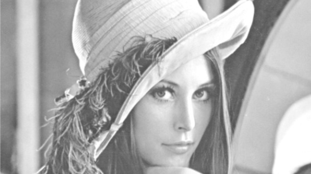
As an example, let’s use an image.
First, convert the image to grayscale (even if it already looks grayscale; in the file you’re loading from, it’s usually stored as a color image).
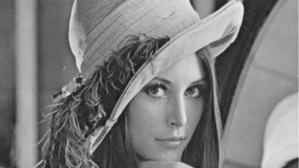
img1 = cv2.imread('imgs/lenna.jpg')
gray = cv2.cvtColor(img1, cv2.COLOR_BGR2GRAY)
We’ll be using the cv2. call repeatedly later on. It’s used to convert between color spaces, for example from BGR to grayscale. Once the image is grayscale, you can add a constant value to it.
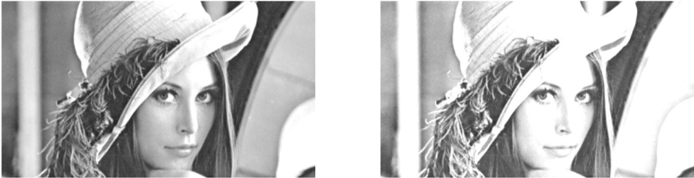
gray_add = cv2.add(gray, 50)
This transformation is equivalent to increasing the image’s brightness.
You can multiply by a factor instead of adding.
gray_mul = cv2.multiply(gray, 1.3)
Multiplying the image is effectively the same as increasing its contrast. You can try a larger coefficient (e.g., 1.).
That’s exactly how brightness and contrast adjustment algorithms work in many popular image editors. However, you can also use more sophisticated functions for this purpose.
Histogram Equalization
A more advanced technique is histogram equalization. Here, a histogram is a representation of an image that shows how many pixels fall into each brightness level. Below is the histogram of a sample image. The black line is the cumulative histogram, which answers the question: how many pixels have a brightness less than x.

As a result of equalization, the image histogram is stretched so that the cumulative histogram approaches a linear function. You can perform the equalization with the following function:
equ = cv2.equalizeHist(gray)
Using our previous figure, the result will look like this.
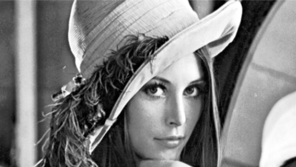
Image Blending
Blending is another example of using simple arithmetic operations on images. If our goal is to combine two images, we could try adding them together. But in that case, when objects overlap, you’ll end up with a mess.
Assume that in one image we know where the object is, and everything else is background. We can then place a second object into the background region. Wherever the second object overlaps the first, the second object takes precedence.
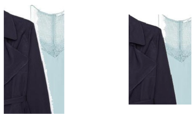
This kind of compositing is sensitive to how cleanly the image is cut out. If the background around the edges isn’t removed properly, you’ll see an ugly white fringe.
It may seem that cleanly cutting an object out of its background is a tough task. It is, because the background is non-uniform—so simply discarding white pixels won’t work. One approach is to use a smart image blending/compositing algorithm and build a mask whose value increases the farther a pixel is from pure white.
Where the original image has white areas, pixels will be taken from the second image, making any rough cutout of the object less noticeable. In the image above, you can see how this simple transformation helps eliminate the problem.
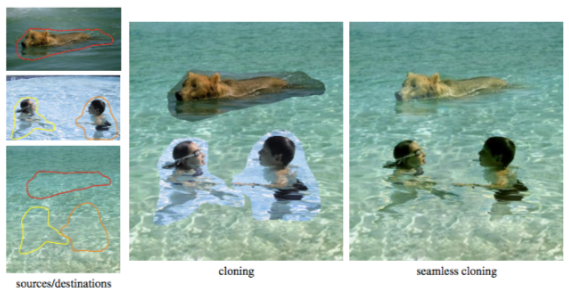
There are more advanced blending algorithms. When you need to copy an object with a non-uniform background and paste it into another image, simple color-mixing methods don’t help. More sophisticated approaches use optimization to figure out what’s object and what’s background. They then transfer the object’s properties unchanged, while taking the background properties from the destination image.
Color spaces
So far we’ve only discussed the RGB representation, but there are other models as well—for example, HSV.
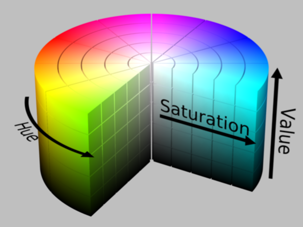
The components of this color space are hue, saturation, and value. It allows you to manipulate color and its saturation independently. Hue represents the pixel’s color and is encoded as a number from 0 to 360, like an angle around a cylinder. Saturation is 0 when the image is grayscale.
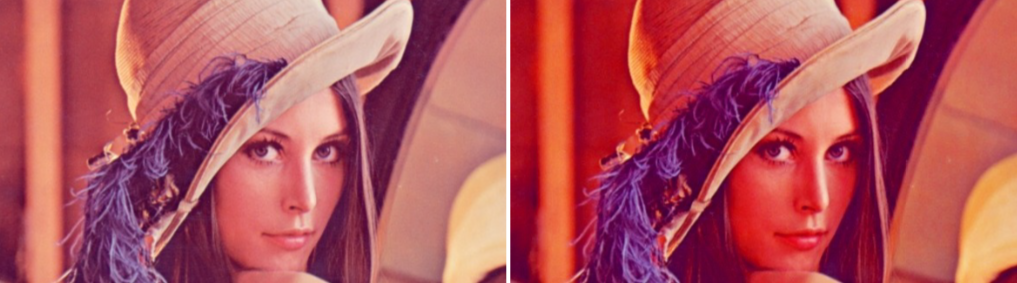
If we’re working with an image in HSV, we can easily make it more saturated by multiplying the saturation channel by a factor. Let’s try increasing the saturation by 50% (a factor of 1.5).
hsv = cv2.cvtColor(img1, cv2.COLOR_BGR2HSV)
hsv[:,:,1] = cv2.multiply(hsv[:,:,1],1.5)
result = cv2.cvtColor(hsv, cv2.COLOR_HSV2BGR)
Haar Cascades for Face Detection
One of the core problems in computer vision is face detection. Among the early approaches, one of the most successful is the Haar cascade method. Using it, you can extract relatively simple features from an image by evaluating patterns formed by several rectangular regions.

Pixels inside the white rectangle are added; those in the black rectangle are subtracted. Sum them up to get a single value. The rectangles and their weights are learned using the AdaBoost algorithm. Since faces have characteristic patterns, a cascade of such filters can then determine whether a face is present or not.
There are face detection methods today that outperform Haar cascades. That said, Haar cascades are simple and widely available off the shelf. If you don’t need top-tier accuracy and just want a quick, easy detector, OpenCV’s Haar cascades are an excellent choice.
Image Segmentation
In general, segmentation isn’t too hard to tackle. One approach is thresholding: assign pixels above a certain cutoff to the object, and those below it to the background.

In this example, the coins are clearly much darker, so it’s enough to choose a threshold that puts all of them below it. Here’s code that does this using OpenCV:
img = cv2.imread('coins.png')
gray = cv2.cvtColor(img,cv2.COLOR_BGR2GRAY)
ret, thresh = cv2.threshold(gray,0,255,cv2.THRESH_BINARY_INV+cv2.THRESH_OTSU)
Linear Image Filtering
One important class of image transforms is linear filters. They’re used for edge and corner detection, as well as for noise removal.
Moving Average as a Convolution
The easiest way to explain linear filtering is with an example. Suppose we need to compute the average over a 3 × 3 window for each pixel. The calculation of this average can be written as follows:
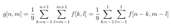
By rewriting the formula as follows, we can derive an expression for the convolution:
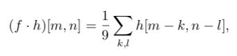
where f is the image (a two‑dimensional function representing the picture), k and l are the pixel coordinates, f(k, l) is the pixel intensity, and h is the convolution kernel (a 3×3 matrix of ones).
When the convolution kernel is a matrix, the operation essentially computes a moving average. In OpenCV, you can perform this convolution as follows:
kernel = np.array([[1,1,1],[1,1,1],[1,1,1]],np.float32) / 9
dst = cv2.filter2D(img1,-1,kernel
As a result, the image becomes blurrier. You can also blur an image by convolving it with a Gaussian function.
cv2.GaussianBlur(img1,(5,5), 0)
 filter, and after Gaussian blur")
Edge Detection
Convolutions can also be used for edge detection. With convolution kernels like the ones shown below, you can extract vertical and horizontal edges. If you combine the results of these two convolutions, you’ll get all the edges.


These kernels are part of the Prewitt operator, and using them is the simplest way to detect edges in an image.
In practice, there are many ways to define boundaries. Each works best under different conditions, so you should choose the method that fits the task at hand.
Correlation
Another example of a linear transformation is correlation. It’s very similar to convolution, but it’s written in a slightly different form:
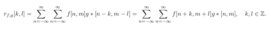
Unlike convolution, correlation measures how similar two images are. This can be used for object detection—for example, to locate a football player’s face.
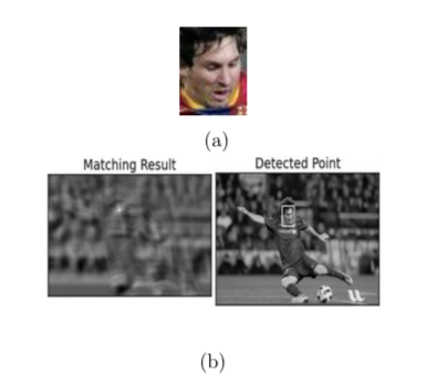
The image on the left shows the result of using correlation for face detection. The white spot marks where the face was found. Correlation can be used with different settings: you can normalize it or use various variants of the method.
So, correlation is a very straightforward way to locate objects in an image, provided you have their exact templates.
Summary
So, we’ve discussed the challenges of pattern recognition and reviewed the basic principles and techniques for working with images. The most important building blocks of deep neural networks are, in fact, convolutional layers. That’s why, when developing ML algorithms for images, it’s essential to understand what a convolution is and what it’s used for. And if you want to cover the rest of the data science fundamentals, you can head over to datasciencecourse.ru, take all five courses, and build your own project under a mentor’s guidance.