Since such devices as bladeRF, HackRF, RTL-SDR, and software systems like GNU Radio had become widely available, reverse engineering of radio air data got really simple and entertaining.

WARNING

All information is provided for informational purposes only. Neither the editorial board nor the author is responsible for any possible harm caused by the materials of this article.

BladeRF, HackRF (to a lesser extent RTL-SDR) make it possible to fully observe the air and interact with it. Some enthusiasts have already created software allowing to interpret GPS signals, set up a Bluetooth stack and Wi-Fi on a computer and launch your own GSM base station. One guy even managed to intercept the signals from the meteorologic satellite and deciphered the transmitted images. Actually, the examples are numerous.

INFO

The similar result can be achieved by connecting a radio transmitter to the audio-card input, but in this case the system will only cover the range around several dozens kilohertz (in accordance with the audio-card’s sampling rate), which is not much and just won’t fit for many tasks.

The default standard option for radio signal investigations software is GNU Radio. This system offers a great set of tools from filters and simple mathematical transformations of the signal to interfaces allowing to transmit data to the network and write your own modules. This soft is what we will use.

INFO

There are quite a few useful modules for GNU Radio. Gr-gsm is definitely worth mentioning, it helps work with GSM networks data.

Installation

We are going to work with OS X. If you don’t have Xcode, you will have to get it from App Storesince we will need the compiler that goes complete with it. Since we are going to use GNU Radio, we’ll also need the graphic system X11 (take it here). Now let’s install the main libraries Macports. If you don’t have them, download them at macports.org):

$ sudo port install bladeRF +tecla

Then you should add the following to the shell config file .bashrc:

export DISPLAY=:0.0
export PATH=/opt/local/bin:/opt/local/sbin:$PATH
export MANPATH=/opt/local/share/man:$MANPATH
export PYTHONPATH=/opt/local/Library/Frameworks/Python.framework/Versions/2.7/lib/python2.7/site-packages:/opt/local/lib/python2.7/site-packages:${PYTHONPATH}

If everything goes well, the response should look more or less like this:

$ bladeRF-cli -p
  Backend:        libusb
  Serial:         d1ece1003730a1a27f9beeba1f511413
  USB Bus:        4
  USB Address:    8

To see full information, enter interactive mode:

$ bladeRF-cli -i

And type info and version:

bladeRF> info
  Serial #:                 d1ece1003730a1a27f9beeba1f511413                          
  VCTCXO DAC calibration:   0x894e
  FPGA size:                40 KLE
  FPGA loaded:              no
  USB bus:                  2
  USB address:              3
  USB speed:                SuperSpeed
  Backend:                  libusb
  Instance:                 0

bladeRF> version
  bladeRF-cli version:        0.11.0-git-58c3ff4
  libbladeRF version:         0.16.1-git-58c3ff4
  Firmware version:           1.7.1-git-ca697ee
  FPGA version:               Unknown (FPGA not loaded)

Here we should pay attention to the following line:

FPGA size:                40 KLE

Important point: for our device to work we’ll need an FPGA image, which you can download for instance from here. Choose a file depending on the FPGA size (we have 40 KLE), in our case it will be hostedx40-latest.rbf. Download it and load using the command

$ bladeRF-cli -l hostedx40-latest.rbf

You should see the lights flickering on the device — this means it is ready for work.

INFO

FPGA — is a semiconductor device that allows hardware realization of various operations such as digital processing of signals and other interesting and useful things. For example, you can use it to set up BladeRF to work without a computer.

The last thing is unstalling GNU Radio, to do it use the following command

$ sudo port install gnuradio +grc +swig +wxgui +qtgui +python27

Then add bladeRF support to GNU Radio using gr-osmosdr module:

$ sudo port install gr-osmosdr

Now you can launch the program and start playing:

$ gnuradio-companion

Tuner to search for an active signal

First let’s make a scanner with a visualization of frequency spectrum to scan the air. It will help us find the signal from the car alarm remote for our research. To do it, choose osmocom Sink inGNU Radio’s right window — it is the model of the device itself — then drag this block to the working area and specify the device in the block’s preferences (we have bladeRF, so in Device Arguments we set bladerf=0). Then put there the frequency (Ch0: Frequency) and bandwidth the scanner will see. Other settings can stay at their default values for now.

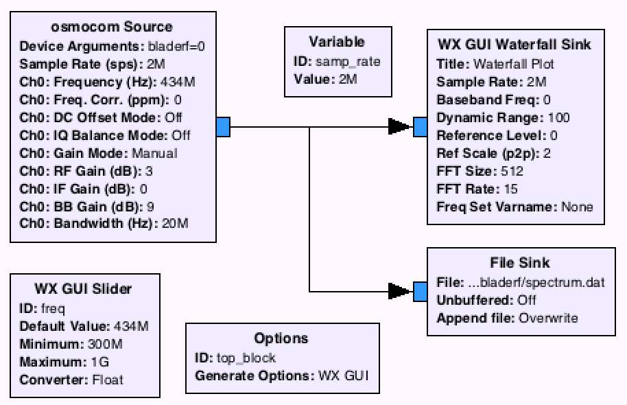
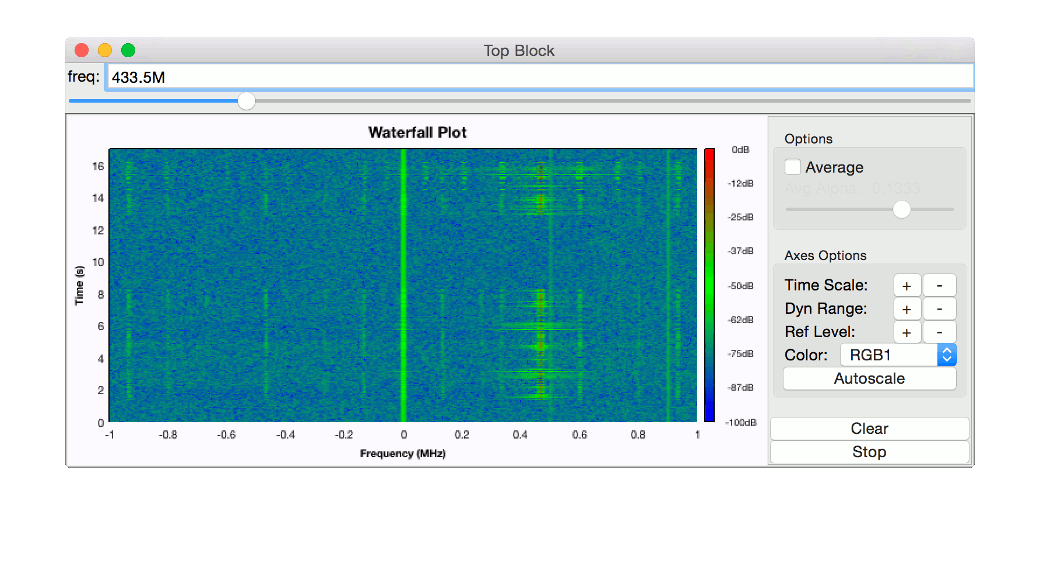
For convenience you would want to place the controls for the frequently used variables straight to your working area — sliders or just boxes with the values. Since we are working with a scanner, let’s put here a slider changing our working frequency in midair (no pun intended): just drag the block WX GUI Slider and set the borders for it, default value and ID, for example, freq. In osmocom Sink in the “Frequency” field we write “freq”. Then, let’s add WX GUI Waterfall Sink block (it shows graphic representation of the signal) and connect it to osmocom Sink with a line. To avoid analyzing the signal on the go, usually it’s a good idea to record it into a file and then play it later, during the analysis stage. To do so we add File Sink block with the name of the file to which all the raw data will be recorded, then we make a link and our scanner is ready! Now we can start it, find the working frequency by moving the slider and make a recording of the signal. Let’s save this scheme as tuner.grc, it should look more or less like one in fig. 1. On fig. 2 you can see our tuner at work.

Fig. 1. Scheme of a tuner for finding an active signal

On a Fig. 2. you can see what was going on in the air between 432,5 and 434,5 MHz during the last 16 seconds. In the middle there is the signal generated by our device’s power source, and to the right there it is — the signal from a car alarm remote! Its harmonics can be found on the other frequencies too. They are lower there and disappear much quicker as the signal source moves away and are much harder to study (can be seen of the picture). They appear due to non-linearity of the elements of the schemе

Fig. 2. Working tuner

Analyzing the signal

Let’s create a new scheme (we named ours radioaudi-reversing.grc) where the signal will be sourced not from bladeRF, but from our recorded file. For this we will give our file’s name to the File Source block. Now the most interesting part. When we convert the results of the previous steps (fig. 2) into a plot signal level against time, its value will be equal to the sum of all the amplitudes in all covered frequencies for each moment of time. So the signal we are going to study has to be separated from the noise. For this we will use Low Pass Filter module, it cuts off the frequencies leaving just the parts to the both sides of the zero frequency in the middle (0 MHz). In our case the middle anyway contains the signal of the reference generator of the receiver, so changing the freq parameter won’t help solve the problem. But the whole spectrum can be shifted by multiplying the signal from osmocom Sink by another one with a frequency equal to the required shift. It’s the math.

To do so let’s add a Multiply block and Signal Source, and send the latter one’s output to the former one’s input together with the File Source’s output. The output from the Multiply block in turn should be sent to Low Pass Filter. Here I am using the cutoff frequency of 10 kHz (value 10e3) and transition width of 1 kHz (value 1e3, this parameter is responsible for how “sharply” the filter cuts off the signal, how blurry the edges would be). Another important parameter — Signal Source frequency — is the value of the shift itself, in other words it’s how far the signal will be shifted. It might be a good idea to put in forward to the working area with a slider just like freq, but named for instance freq_0. Now we just direct the Low Pass Filter output straight to WX GUI Waterfall Sink — the meaningful signal should now be right around the middle, at conditional frequency of 0 MHz.

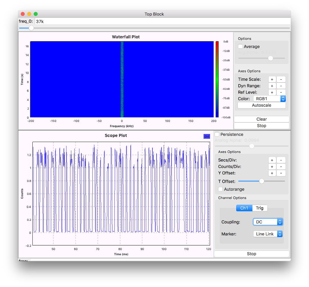
Great! At this point we are really close to actually analyzing the signal. Let’s drag WX GUI Sink to your working area and connect it with the Multiply output through the block named Complex to Mag which transfers signal values from the complex domain to the absolute values domain more convenient to work with. See fig. 3 for reference. It’s a good thing that we have data transferred with amplitude modulation and there are only two levels, so we can have binary representation right away. To do so, direct the output from Complex to Mag to the Binary Slicer block, that converts the sequence of amplitudes into the sequence of zeros and ones, based on values being above or below zero. Since we have only positive amplitudes, let’s lower the curse so that Binary Slicer had positive and negative values to work with. Simple arithmetic block Add const with the value of -170 will do the job. The Binary Slicer’s output goes to the file via File Sink.

In practice the scheme would normally have more modules, including Rational Resampler and Throttle. The former lowers signal sampling rate, to leave out the excessive data, the latter lowers the processor load in a similar way in cases when there is no need to process the entire data flow (like in our case, we only need the data displayed on the screen, that’s all). It would be correct to use Frequency Xlating FIR Filter block, but we used Multiply just for clarity. See final scheme for working with the recorded signal in fig. 4.

Fig. 3. View of the signal as the amplitude versus time plot

Fig. 4. Scheme for working with the signal

Data interpretation

Well, we have got the file containing the bytes representing the signal as a binary sequence. 0x01 for one and 0x00 for zero. Let’s write a simple script in Python to read it. Out script will interpret each sequence of ones and zeroes exceeding a certain threshold as 1 or 0 and separate signals from each other.

#!/bin/python
import sys

f = open("audi.bin")

count1 = 0
count0 = 0
count = 0
signals = []
distinctSignal = []

cc = 0
byte = f.read(1)
sys.stdout.write('Signals in bin:')
while byte:
    byte = f.read(1)
    cc = cc + 1
    if byte == '\x00':
        count0 = count0 + 1
        if count1 > 10:
            if count1 > 600:
                sys.stdout.write('\n')
                cc = 0
                signals.append(distinctSignal)
                distinctSignal = []
            elif count1 > 300:
                sys.stdout.write('1')
                distinctSignal.append(1)
            else:
                sys.stdout.write('0')
                distinctSignal.append(0)
        count1 = 0
    if byte == '\x01':
        count1 = count1 + 1
        count0 = 0
f.close()


# print valid signals

def processSignal(signal):
    if len(signal) < 64:
        return
    n = 0
    hexString = ''
    while len(signal) >= 8:
        n = signal[7] * 1 + signal[6] * 2 + signal[5] * 4 + signal[4] * 8 + signal[3] * 16 + signal[2] * 32 + signal[1] * 64 + signal[0] * 128
        hexString = hexString + ('%02x' % n)
        signal = signal[8:]
    print hexString

sys.stdout.write('\nValid signals in hex:\n')
prev = signals[0]
for signal in signals:
    if signal != prev:
        processSignal(signal)
    prev = signal

In hexadecimal notation we will get the following sequences:

2e23a99426bd8018
2e23a929426b805e
2e23a91f29428039
2e23a9031f298058
2e23a9cf031f809e
2e23a932cf0380b3
2e23a90132cf80b1
2e23a9ab013280f6
2e23a9fab0138040
2e23a90fab0180c8
2e23a9a0fab080fc
2e23a94a0fab80a7
2e23a9234a0f802b
2e23a9a234a08022

Here we clearly see that the information of each signal is transmitted as an 8 byte sequence, where the first three are invariable and make up a preamble, and the other five vary in some unclear pattern.

INFO

With some systems using authorization schemes based on Rolling code you can use jamming: the signal from an active alarm remote is intercepted and at the same time jammed so that the receiver does not get it and more importantly does not consider it invalid. This allows us to use this signal in the future.

Conclusion

As we see, car alarm is pretty well secured because there are 2^(5 8) or one trillion possible variants for exhaustive search. How long would this search take? For one signal sequence there will be about 45 000 measurements of 0 and 1, which together with 400 kHz sampling rate (after decimation of the initial 2 MHz via Ration Resampler) will give us 45 000 (1/400 000) = 0,1125 s. So total search time (given the signals will go one after another) will be 0,1125 * 10^12 ~ 1,125^11 s ~ 3500 years.

Knowing this, one should rather work towards narrowing the search or speeding up the process. Will the independent researchers find a way? Time will show. Good luck in your research!